Chapter 17. Non-linear Regression Analysis
Higher category: 【Statistics】 Statistics Overview
2. polynomial regression model
5. interaction
1. quadratic regression model
⑴ formula

⑵ determination of coefficients
① multiple linear regression model is used : consider Xi and Xi2 as different variables and interpret them
② it is possible because Xi and Xi2 do not have perfect multi-collinearity
⑶ linearity test

⑷ confidence interval of the amount of change
① effect: the effect of Y by a unit change of X is as follows

② marginal effect

③ standard deviation of the amount of change

④ confidence interval of the amount of change

2. polynomial regression model
⑴ general equation

⑵ determination of coefficients : multiple linear regression model is used
⑶ linearity test

⑷ decision of degree (order) of polynomial 1. top-down method
① the most commonly adopted method
② 1st. set the maximum value of r
③ 2nd. test H0 : βr = 0
④ 3rd. if H0 is rejected, r is the degree of regression line
⑤ 4th. if H0 is not rejected, eliminate Xir and repeat 2nd step for βr-1, ···
⑸ decision of degree (order) of polynomial 2. bottom-top method
① a way to see if there is a significant effect on explaining a given sample when a term with a higher order of one level is added
② procedure
○ 1st. assume that the coefficient for all terms is significant up to the (r-1)-order polynomial of in the botom-top manner
○ 2nd. add a r-order term
○ 3rd. calculate the sum of squares by the r-order regression line (degree of freedom: r)
○ 4th. subtract the sum of squares by the (r-1)-order regression line (degree of freedom: r-1) from the value obtained from 3rd step
○ 5th. calculate the sum of squares by the residual of the r-order regression line (degree of freedom: n-1-r)
○ 6th. calculate the mean square by dividing the value obtained from 5th step by (n-1-r)
○ 7th. divide the difference of the sum of squares obtained from 4th step by the mean square obtained from 6th step: the degree of freedom of the difference of the sum of squares is 1
○ 8th. calculate p value by substituting F statistic obtained in 7th step from F(1, n-1-r)
③ example
○ problem situation
| model | sum of squares | df | mean square |
|---|---|---|---|
| linear | 3971.46 | 1 | 3971.46 |
| error | 372515.09 | 18 | 20695.28 |
| quadratic | 367833.58 | 2 | 183916.79 |
| error | 8652.97 | 17 | 509.10 |
| cubic | 369211.71 | 3 | 123070.57 |
| error | 7274.84 | 16 | 454.68 |
Table 1. problem situation
○ table of results
| model | difference of sum of squares | df | sum of squares of residuals | df | mean of sum of squares of residuals | F ratio |
|---|---|---|---|---|---|---|
| quadratic | 367833.58 | 2 | 8652.97 | 17 | 509.10 | F1,17 = 714.72 |
| linear | 3971.46 | 1 | p < 0.001 | |||
| difference | 363862.12 | 1 | ||||
| cubic | 369211.71 | 3 | 7274.84 | 16 | 454.68 | F1,16 = 3.03 |
| quadratic | 367833.58 | 2 | NS | |||
| difference | 1378.13 | 1 |
Table 2. table of results
④ drawbacks: sequential type Ⅰ error accumulation is problematic
○ the study of statistics is to analyze them with a phenomenon that occurs at once
○ it’s very difficult to analyze a phenomenon of a certain probability by applying another phenomenon that has already appeared with a different probability
○ difficulty means that the statistic may not follow the F distribution
○ bottom-top method of degree determination is to analyze a phenomenon of a different probability in a phenomenon of a particular probability
○ the phenomenon of a particular probability refers to the (r-1)-order regression equation
○ the phenomenon of a different probability refers to the r-order regression equation
○ (note) it is impossible to clearly show the difference of sum of squares follows the F distribution
3. logarithm regression model
⑴ (note) logarithmic approximation

⑵ class 1. linear-log model
① formula

② if Xi increases by 1%, Yi increases by 0.01β1
⑶ class 2. log-linear model
① formula

② if Xi increases by 1,Yi</sub increases by 100β1%
⑷ class **3.** log-log model
① formula

② if Xi increases by 1%, Yi increases by β1%
⑸ we can select the more appropriate model by compairing adjusted R2 between log-linear model and log-log model
⑹ it’s pointless to compare linear-log model with other two models, as the dependent variable of linear-log model differs
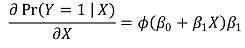
4. probability model: the case of dependent variable being a binary variable
⑴ linear probability model (LPM)
① formula
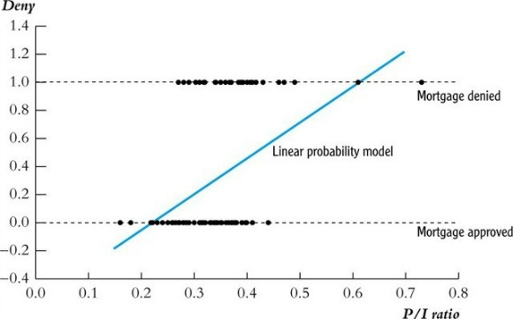
Figure 1. linear probability model

② issue : the dependent variable does not always show values between 0 and 1
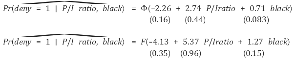
⑵ probit regression model
① overview : the most frequently used probability model
② formula
○ simple model
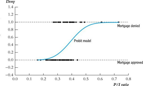
Figure 2. probit regression model
○ multiple model

③ effect
○ formula

○ marginal effect
④ statistical estimation
○ there is no exact form of function of the estimator of each coefficient : find the maximum likelihood estimator through numerical analysis
○ once obtained, the maximum likelihood estimator satisfies consistency and normality
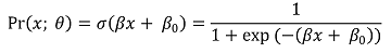
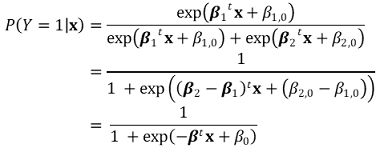
⑶ logistic regression model
① formula
○ logistic function
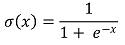
○ modeling: put the linear regression form of βx + β0 to logistic function, which is a kind of a linking function
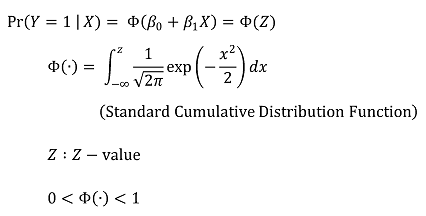
○ log-odd (logarithmic of odds ratio) : also called logit. A logarithmic conversion of the odds ratio. having a value from negative to positive infinity.
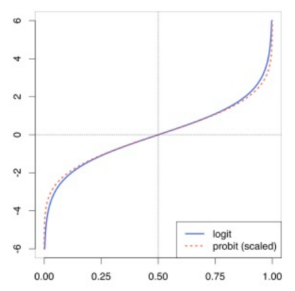
Figure 3. logit function
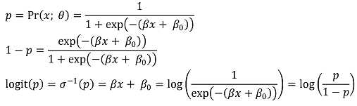
○ The logistic function is the inverse function of the logit function.
○ The logistic function transforms an input variable that takes values from negative infinity to positive infinity into an output variable that ranges from 0 to 1.
○ assume the independent variable is not ome-dimensional variable of xi but multidimensional variable of xi, and use the Bernoulli function
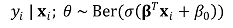
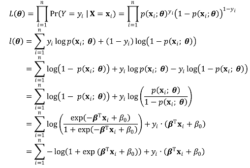
○ definition of likelihood function of L(θ) and log likelihood function of ℓ(θ) : here, L(θ) is defined as a cross-entropy
○ lemma : L(θ) and ℓ (θ) are convex function. the minimal solution is not local solution but global solution. proof is complicated
○ step 1. definition of gradient
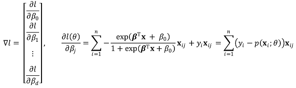
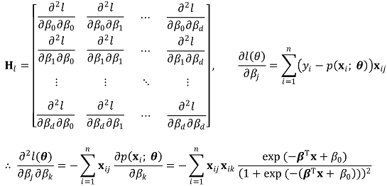
○ step 2. definition of Hessian matrix
○ step 3. get the Taylor series for θk for the secondary approximated equation and obtain the maximum solution θk+1 = θk + dk of the approximated equation
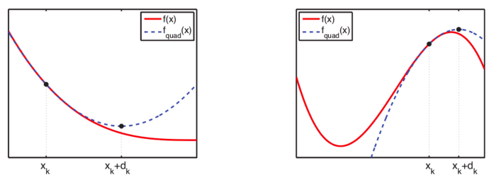
Figure 4. relationship between maximum likelihood estimation and Taylor series
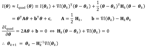
○ step 4. updating θk in a way of Newton-Raphson method reaches the global maximum
○ this is obtained by numerical analysis, but does not have the exact function form of the estimator of each coefficient.
③ idea for the proof of consistency (assuming symbols may differ from the above)

④ idea for the proof of asymptotic normality (assuming symbols may differ from the above)

⑤ application : multiclass classification
○ intoduction: as logistic regression is a binary classification, it cannot be applied directly to multiclass classification
○ method 1. performing 1 vs {2, 3} at first, and 2 vs 3 afterward
○ method 2. softmax function
○ definition
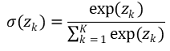
○ softmax function in multiclass classification
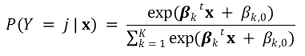
○ proof : logistic regression is a special example of softmax function
⑷ Comparison of LPM, probit, and logistic function
① unable to compare coefficients between LPM, probit, and logistic because models are different
○ example 1. comparison between probit regression model and logistic regression model
○ showing very similar plots
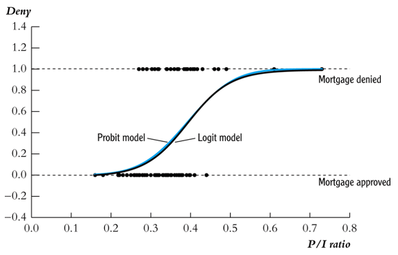
Figure 5. comparison between probit regression model and logistic regression model
○ the difference in coefficients is very significant: there is no mathematical meaning to this difference
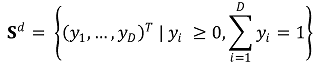
⑸ Dirichlet regression model:
① Overview : Used for regression analysis while considering the topology (simplex) of the data.
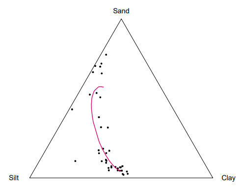
Figure 6. Situations where the Dirichlet regression model is applied
② Sample space: A multi-dimensional vector representing the proportions or probabilities of each item
</br>
○ Non-negative data
○ Unit-sum
○ D: The number of components, i.e., the size of the dimension
○ d = D - 1
③ Dirichlet distribution: Gains attention because it can analyze the simplex.
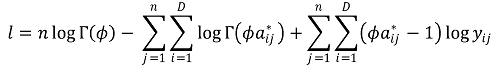
④ Estimation of Dirichlet regression:
○ Aitchison (2003) first introduced the log-ratio transformation.
○ Log-likelihood function: Given n data points,
</br>
○ Zero data can be a problem in the log-likelihood function.
○ Solution 1: Replace zero data with very small nonzero values, as proposed by Palarea-Albaladejo, Martín-Fernández, and others.
○ Solution 2: Use a dual model that handles zero data separately, as proposed by Zadora, Scealy, Welsh, Stewart, Field, Bear, Billheimer, and others.
○ Solution 3: Use an improved regression model that robustly applies to zero data, as proposed by Tsagris, Stewart, and others.
5. interaction
⑴ modeling
① interaction regressor or interaction term is introduced

② unable to compare coefficients with models without interaction terms
③ 3 or more multiple interactions can also be defined
⑵ effect: the change of Yi by a unit change of Xi is as follows

⑶ elasticity
① intuitively, it means the degree to which the absolute value of the slope is large
② in microeconomics, elasticity means the slope multiplied by (-1)
⑷ applicatio n: interaction of binary variables
① modeling

② effect : the effect of Y by a unic change of X is as follows

③ H0 : the proposition that Y is not affected by D can be tested by F statistic concerning β2 = β3 = 0. determinant check
④ H0 : the proposition that the effect of Y by a unit change of X is not affected by D can be tested by t statistic concerning β3 = 0
⑤ the entire regression line can be obtained by using the regression line of D = 0 and the regression line of D = 1

⑸ application: interaction of two binary variables (dummy variables)
① modeling

② knowing 2 × 2 table for D1, D2 can lead to regression line equation
Input : 2019.06.21 12:10