Korean, Edit

Chapter 9. Theorems of Statistics I

Higher category: 【Statistics】 Statistics Overview

1. Markov inequality

2. Chebyshev inequality

3. Cantelli inequality

4. Cauchy-Schwarz inequality

5. Jensen inequality

6. Law of large numbers

7. Central extreme theorem

8. Slutsky’s theorem

9. Laplace’s rule of succession

a. Collective wisdom

1. Markov inequality

⑴ theorem 

when X is the random variable and a > 0, the following is established:

⑵ proof 1.

let x₁, ···, x_n be events that make up the random variable X. by reordering the events, we can acquire | x_i | ≥ a ⇔ i = r+1, ···, n

⑶ proof 2. 

2. Chebyshev’s inequality 

⑴ theorem

there is a random variable with expected value of m and variance of σ².  the variance is a finite value. then, for any real number k ＞ 0, the following inequality is established: 

however, meaningful information is provided only when k>1.

⑵ proof 1. 

let x₁, ···, x_n be events that make up the random variable X. by rearranging the above events, we can acquire | x_i - m | ≥ kσ ⇔ i = r+1, ···, n. 

⑶ proof 2. 

the case of Markov inequality with k = 2, ε = kσ, X → X - μ_X is Chebyshev’s inequality 

3. Cantelli inequality (one-tailed chebyshev inequality) 

⑴ theorem

there is a random variable with expected value of m and variance of σ². the variance is a finite value. then, for any real number k ＞ 0, the following inequality is established: 

⑵ proof 

① m = 0

let x₁, ···, x_n be events that make up the random variable X. by reordering the events, we can acquire x_i ＜ kσ ⇔ i = r+1, ···, n. if we put kσ = t,

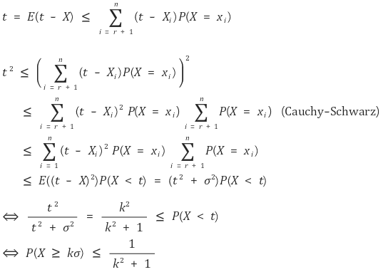
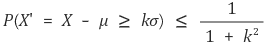
② m = μ ≠ 0 

X’ = X - μ is a random variable with an expected value of 0 and a variance of σ². so the following is established:

4. Cauchy-Schwarz inequality 

⑴ theorem

⑵ proof 

⑶ example 

① E(1 / X) ≥ 1 / E(X)

② ln (E(X)) ≥ E(ln X)

5. Jensen’s inequality 

⑴ convex function and concave function

① convex set: it refers to the case where the internally dividing points of any two points in a set are always elements of the set

② convex function: the function where ｛(x, y) y ≥ f(x)｝ is a convex set. it is similar to ‘convex downward’

③ strictly convex function

④ concave function: the function where｛(x, y) y ≤ f(x)｝is a convex set. it is similar to ‘convex upward’

⑤ strictly concave function 

⑥ linear function: the case of both covex function and concave function

⑵ relationship between convexity and the secondary derivative: f”(x) ≥ 0 and the convex function are necessary and sufficient. f”(x) ≤ 0 and the concave function are necessary and sufficient

① proof 1. 

② proof 2. an easy proof showing that for the convex function, f”(x) ≥ 0 is established and for concave function, f”(x) ≤ 0 is established 

⑶ Jensen’s inequality: expansion of dimension 

① when f is a convex function, the following inequality is established:

② when f is a concave function, the following inequality is established: 

③ proof 1. mathematical induction

④ proof 2. introduction of a linear function.

○ proof 

let’s define ℓ(x) as a straight-line function that passes (E(X), f(E(X)), and tangles f(x). let’s say f is a convex function. then,

⑷ economic statistical meaning.

① risk-loving

○ convex function

○ if the utility function for the mean is smaller

○ if you prefer adventure

② risk-avoiding 

○ concave function

○ if the utility function for the mean is greater

○ if you prefer predictable results

③ risk-neutral

6. law of large numbers (LLN)

⑴ theorem

for any real number α > 0, the following equation is established:

⑵ proof 

suppose the mean of the random variable X is m, and the standard deviation of it is σ. for any real number k > 0, let’s apply Chebyshev inequality 

⑶ sufficient condition

① the random variable Xi, i = 1, ···, n is i.i.d

② VAR(X_i) ＜ ∞ 

⑷ Application

① Weak Law of Large Numbers (Weak LLN, WLLN)

○ Convergence in probability

○ Guarantees that the probability of the sample mean approaching the expected value converges to 1.

○ In other words, it only ensures that the likelihood of the sample mean getting close to the expected value increases in a probabilistic sense.

② Strong Law of Large Numbers (Strong LLN, SLLN)

○ Convergence almost surely: If this holds, convergence in probability naturally follows.

○ Guarantees that in almost all cases, the sample mean will certainly converge to the expected value.

○ In other words, even when looking at individual realizations, it ensures that the mean ultimately converges to the expected value.

7. central limit theorem (CLT)

⑴ outline

① definition: when the number of samples is infinitely large, the sample sum and sample mean are normally distributed regardless of the distribution of the samples

② mathematical expression: uses convergence in distribution

⑵ Proof 1.

if the probability of an event occurring is p, the probability of an event occurring k times during n trials is as follows:

as n approaches infinity, this probability distribution changes almost continuously. therefore, we can think of the following function, which takes the real value as the domain of x

① average

if f has the maximum value at the point of x = m in the distribution, the following equation is established:

pay attention to the next

however, the Sterling approximation can strictly prove that the definition of n! is as follows

therefore

② normal distribution approximation of the binomial distribution

for Δx = x - m that is small enough, the following holds true

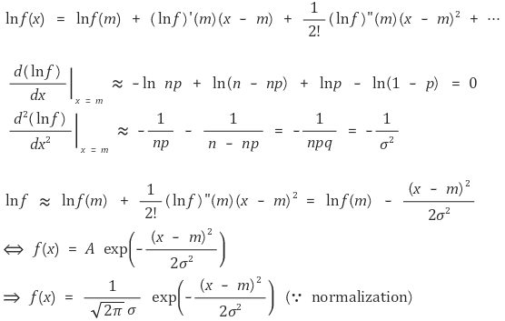
as a result, B(n, p) is close to N(np, npq) around the average (assuming, n ≫ 1)

⑶ proof 2. introduction of m(t) and moment generating function 

⑷ sufficient condition 

① X_i, i = 1, ···, n is i.i.d

② 0 ＜ VAR(X_i) ＜ ∞

⑸ Application

① Conditions for Normal Approximation of Binomial Distribution: Variance = npq ≥ 10

② Conditions for Normal Approximation of Poisson Distribution: λ ≥ 30

⑹ Example problems for central limit theorem

8. Slutsky’s theorem 

⑴ convergence in probability: for random variables S1, S2, ···, Sn, 

⑵ convergence in distribution: for random variables S1, S2, ···, Sn, for each distribution function F1, F2, ···, Fn, and for S that takes F as its distribution function,

⑶ Slutsky’s theorem (algebra of probability limit): when there exist p lim Xn, p lim Yn, 

① the above 6-th formula is called CMT (continuous mapping theorem)

9. Laplace’s rule of succession

⑴ definition: when k positive results are obtained during n trials, the probability of the positive result in the n+1-th trial is as follows

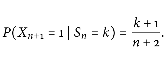
⑵ proof (refhttps://jonathanweisberg.org/pdf/inductive-logic-2.pdf)

Input : 2019.05.03 15:02