Korean, Edit

Chapter 13. Statistical Estimation

Higher category : 【Statistics】 Statistics Overview

1. overview

2. point estimation

3. interval estimation

1. overview 

⑴ statistical estimation: estimating the characteristics of a population through samples

⑵ state space: ℝn. a set of all the observed samples 

2. point estimation (parametric approach, location type)

⑴ definition: estimating parameters from samples (x₁, ···, x_n)

① parameter : values showing the characteristics of the population. μ, σ, θ, λ, etc

② μ : mean of population

③ σ : standard deviation of population

④ θ : θ: probability of success in Bernoulli distribution or binomial distribution

⑤ λ : λ of Poisson distribution or exponential distribution

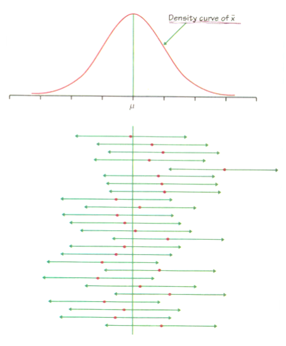
⑵ sampling distribution (empirical distribution)

⑶ point estimator: for parameter θ, 

① definition 1. point estimator is not a single number but a function

② definition 2. point estimator is a function for X₁, ···, X_n 

③ definition 3. the probability of a point estimator is a function of θ

⑷ criteria for a good point estimator 

① expected error or mean squared error (MSE) : also called model risk

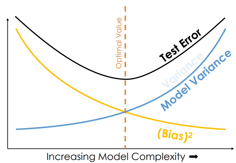
○ bias-variance decomposition 

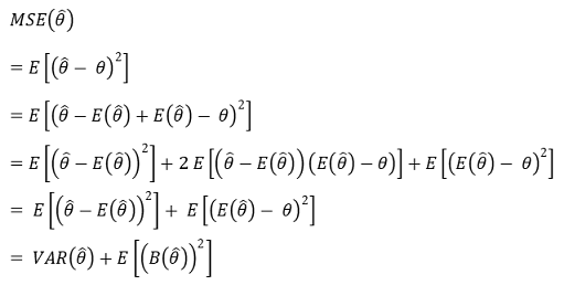
○ as the covariance of bias and chance error is 0 intuitively, we can remove the intermediate term 

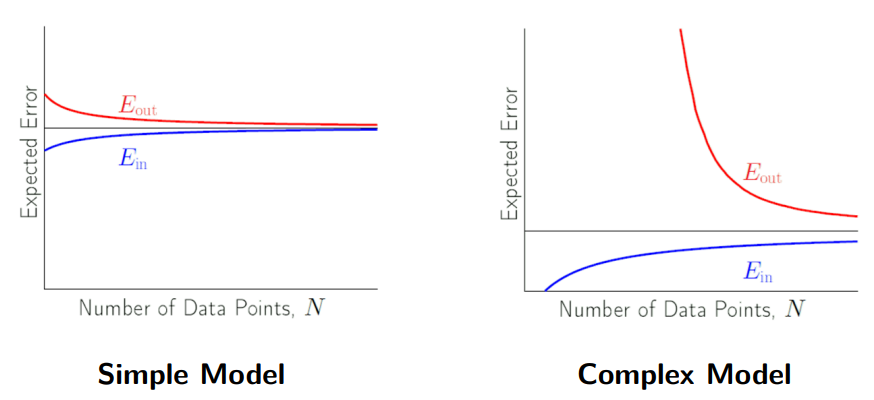
○ the strategy to reduce the bias increases the model variance

○ the strategy to reduce the model variance increases the bias

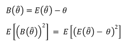
② criterion 1. bias: also called systemic error, non-random error, and model bias

○ small bias required

○ cause: underfitting, lack of domain knowledge

○ solutions: use of more complex models, use of models suitable for domain

○ unbiased estimator: B = 0 ⇔ sample mean = population mean. if there’s unbiasedness, it’s a good estimator

○ example 1. sample mean: unbiased estimator of population mean 

○ example 2. sample variance : unbiased estimator of population variance 

○ example 3. sample covariance

○ example 4. when X_i ~ u[0, θ], either unbiased estimator or not 

③ criterion 2. efficiency: related to random chance error

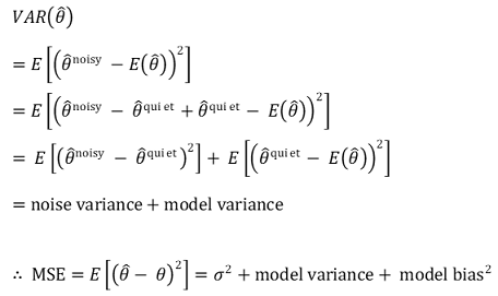
○ small variance is required based on the premise of unbiased estimator  

○ 2-1. noise variance: also called 1st chance error and observation variance. marked as σ²

○ example : error of the instrument itself, noise of the target itself

○ there are attempts to measure these information, but there are many difficulties

○ 2-2. model variance: also called 2nd chance error

○ chance error due to the fact that the sample group is a randomly extracted set from the population

○ cause : overfitting

○ solution : using a simpler model

○ bias-variance tradeoff : as model complexity increases, the bias decrease, but model variance increases, resulting in trade-off relationship and optimal complexity

○ BLUE (best linear unbiased estimator) : the estimator of the smallest variance among linear unbiased estimators

○ uniformly minimum variance unbiased estimator (UMVU)

○ definition: the estimator of the smallest variance among unbiased estimators including non-linear unbiased estimators 

○ the direct calculation of Fisher information In 

○ the indirect calculation of Fisher information In  

○ Cramér–Rao lower bound = 1 / In

○ if an estimator is equal to the Cramér–Rao lower bound, it is UMVU 

④ criterion 3. consistency and consistent estimator 

○ asymptotic property: characteristic of sample, of which size is approaching ∞

○ asymptotic unbiasedness: the case in which the unbiasedness is established when n → ∞. it is related to the law of large numbers

○ asymptotic efficiency 

○ consistency : the property of the estimator converging into a parameter

○ X is a random variable, but generally considered as a specific constant

○ example: the following is a poor random variable because it is inconsistent

⑤ criterion 4. least squared estimator

⑸ method 1. discrete probability distribution and maximum probability

① it uses the definition of binomial coefficients

② example

○ situation: number of members of a population are estimated through marking-and-recapture method

○ given the number of members N, the number of firstly captured members m, the number of lastly captured members n, the number of lastly marked memebers x

○ probability distribution: hypergeometric distribution

○ question: the most reasonable value of N 

⑹ method 2. method of moment estimator (MOM): also called sample analog estimation

① definition: the method of calculating the estimator of θ in a way of θˆ =g^-1((1/n) × ∑X_i^k) based on the fact that E(X^k) = g(θ) ⇔ θ = g^-1(E(X^k)) 

○ E(X^k) : moment or population moment

○ (1/n) × ∑X_i^k : sample moment

○ the moment is a constant, and the sample moment is a random variable with a constant distribution

○ consistency : by the law of large numbers, the sample moment converges into the moment 

② sample moment

○ k-th order sample moment for origin

○ k-th order sample moment for sample mean

③ example

⑺ method 3. maximum likelihood method (ML) 

① definition

○ θ : parameter

○ θ* : the estimator of the parameter θ

○ θ_ML : the maximum likelihood estimator of the parameter θ

② likelihood: the possibility of something happening

③ likelihood function

○ the probability that a given sample will come out when θ* is given.

○ also known as product of likelihoods

○ that is, p(X | θ*)

○ marked as ℒ

④ log likelihood function: taking a log into the likelihood function

○ marked as ℓ = ln ℒ

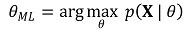
⑤ maximum likelihood estimation: examining θML that maximizes the likelihood function p(X | θ)

○ assumption : the closer the θ* is to parameter θ, the greater the likelihood function will be

○ 1^st. differentiation of log likelihood function: acquire θ* that makes the local maximum on a valid interval 

○ 2^nd. if the local maximum exists: it is assumed that the θ* that makes the local maximum is θML 

○ 3^rd. if the local maximum doesn’t exist: it is assumed that θ* with higher likelihood of both ends of a valid interval is θML 

○ maximum likelihood estimation and Hessian matrix: a useful method for obtaining estimators of all differentiable functions

○ step 1. get the second order approximation by obtaining the Taylor series for θk , and calculate the solution θ_k+1 = θ_k + d_k that maximize the approximated equation 

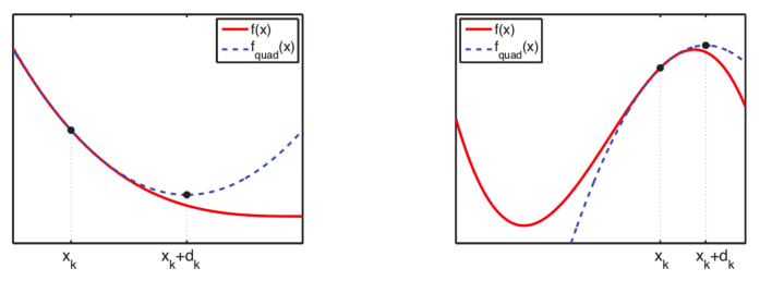
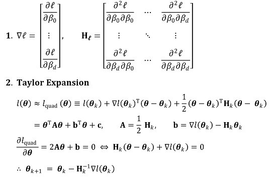
○ step 2. Newton-Raphson method : updating θ_k will eventually reach the global maximum

○ example : logistic regression 

⑥ maximum likelihood estimator : when sample X is given, the function G corresponding to θML that maximizes the likelihood 

○ θ_ML = G_ℓ (ℓ) = G_ℒ(ℒ)

○ limitation of the estimator: there are limits on the assumption of maximum likelihood estimation

○ the estimator favored by statisticians.

⑦ example 1.

⑧ example 2.

⑨ example 3. 

⑩ example 4. the maximum likelihood estimation might not be determined solely

⑪ characteristic 1. consistency

⑫ characteristic 2. asymptotic normal distribution

⑬ characteristic 3. invariance : if θ_ML is the maximum likelihood estimator of θ, g(θ_ML) is the maximum likelihood estimator of g(θ)

⑭ characteristic 4. the maximum likelihood estimation is a special example of Bayes rule 

3. interval estimation (scaling type) 

⑴ definition: estimating which interval the parameter is in through the samples 

① purpose of introduction: the probability that the point estimator exactly matches the actual parameter is zero

② confidence level (confidence coefficient)

○ P(θ_left ＜ θ ＜ θ_right) = 1 - α, 0 ＜ α ＜ 1

○ threshold: values that constitute the boundary of the confidence interval. θ_left, , θ_right, etc 

○ 1 - α : confidence level (confidence coefficient)

○ α : rejection probability or significance level

○ confidence interval: the interval [θ_left, θ_right] , the probability of θ being on which is (1 - α) × 100%

③ notes

○ P(Z ＞ 1.65) = 5% ⇔ P( Z ＞ 1.65) = 10%

○ P(Z ＞ 1.96) = 2.5% ⇔ P( Z ＞ 1.96) = 5%

○ P(Z ＞ 2.58) = 0.5% ⇔ P( Z ＞ 2.58) = 1%

④ 68 - 95 - 99.7 rule 

○ μ ± 1 × σ : 68.27 %

○ μ ± 2 × σ : 95.45 %

○ μ ± 3 × σ : 99.73 %

⑵ case 1. when Xi ~ N(μ, σ²) and the population variance σ² is known 

① overview: a normal distribution is used

② method

○ introduction: when μ is known, the probability of X_avg (confidence level : α) is as follows

○ change of ideas: X_avg ∈ I (μ) ⇔ μ ∈I (X_avg) (confidence level: α)

○ meaning : it means the probability distribution of μ when X_avg is known 

○ it is noted that the probability distribution of μ follows the same conceptual framework of the probability distribution of X_avg when μ is known 

○ draw your own picture to confirm

○ pivotal estimation : for the shortest confidence interval, it should be established that |a| = |b|, i.e. a = -z_α/2, b = z_α/2. here, the proof is omitted

③ if you know the distribution function

○ example 1. F(x) = √x / θ, 0 ≤ x ≤ θ² : the 90% confidence interval is as follows

○ example 2. F(x) = (x / θ)ⁿ : the 90% confidence interval is as follows

⑶ case 2. when X_i ~ N(μ, σ²) and the population variance σ² is unknown 

① overview 

○ normal distribution needs to know the variance of the population 

○ in reality, the sample variance is used because the population variance is unknown 

○ the distribution of sample mean when using sample variance instead of population variance is exactly t-distribution 

② example 1. sample mean

○ introduction: when μ is known, the probability of X_avg (confidence level : α)

○ change of ideas : X_avg ∈ I* (μ) ⇔ μ ∈ I* (X_avg) (confidence level : α)

○ pivotal estimation: for the shortest confidence interval, it should be established that |a| = |b|, i.e. a = - t_α/2, b = t_α/2. here, the proof is omitted

③ example 2. (case 1) when X_i (μ_X, σ²) (i = 1, ···, n) and Y_j (μ_Y, σ²) (i = 1, ···, n) are paired 

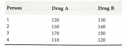
○ also called paired estimation (matched sample estimation)

○ in fact, there is only one variable: after defining W_i = X_i - Y_i, manipulate example 1 

○ an example of a paired sample 

○ an example of an independent sample 

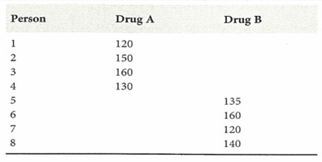
④ example 3. (case 2) difference of two sample means : when X_i (μ_X, σ²) (i = 1, ···, n) and Y_j (μ_Y, σ₂) (j = 1, ···, m) are independent 

○ when the variances of two sample means are same in unpaired sample estimation (pooled sample estimation) 

○ formula 

○ confidence interval for confidence level α

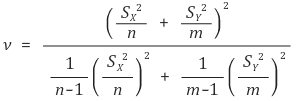
⑤ example 4. (case 3) difference of sample means: when X_i (μ_X, σ_X²) (i = 1, ···, n) and Y_j (μ_Y, σ_Y²) (j = 1, ···, m) are independent (assuming σ_X ≠ σ_Y)

○ when the variances of two sample means are different in unpaired sample estimation (pooled sample estimation) 

○ Welch approach is used

○ degree of freedom in (case 3) is lower than (case 2) → power of test decreases

○ the formula of ν is very complex

⑥ example 5. confidence interval of population variance 

○ note that there is no obvious solution in minimizing the size of the confidence interval: numerical analysis should be used

○ the given model

○ confidence interval for confidence level α

⑦ example 6. ratio of population variance

○ confidence interval for confidence level α

⑷ case 3. when samples do not follow normal distribution, but there are many samples

① central limit theorem : if n is large enough, the distribution of sample mean converges into normal distribution

○ formula

○ t distribution eventually converges into normal distribution

② number of samples

○ normality is typically achieved with only 25 ~ 30 samples

○ for a symmetric unimodal distribution (having one extreme value), n = 5 is sufficient

③ example 1. population ratio

○ given model

○ confidence interval for confidence level α 

④ example 2. correlation coefficient 

○ null hypothesis H₀ : correlation coefficient = 0

○ alternative hypothesis H1 : correlation ceofficient ≠ 0

○ calculation of t statistics: for the correlation coefficient r obtained from the sample,

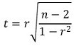
○ the above statistic follows the student t distribution with a degree of freedom of n - 2 (assuming the number of samples is n)

Input : 2019.06.19 14:23