Korean, Edit

Chapter 16. Linear Regression Analysis

Higher category: 【Statistics】 Statistics Overview

1. regression analysis

2. simple linear regression model

3. multiple linear regression model

a. Regression Analysis in R

–

1. regression analysis 

⑴ regression analysis: representing a particular variable as a dependency of one or multiple other variables

① more precisely, y ~ X (assuming y ∈ ℝ) 

○ included in a supervised algorithm

○ (note) Classification: y ~ X (assyming ㅣ { y }

＜ ∞ )

○ (note) Engression: While general regression assumes Y = g(X) ± ε, engression instead models Y = g(X + ε), which makes extrapolation possible (where ε is noise).

② Specific variables: The name dependent variable is representative, but there are several names

○ Response variable

○ Outcome variable

○ Target variable

○ Output variable

○ Predicted variable

③ Other variables: The name independent variable is representative, but there are several names

○ Experimental variables

○ Explanatory variable

○ Predictor variable

○ Regressor

○ Covariate

○ Controlled variable

○ Manipulated variable

○ Exposure variable

○ Risk factor

○ Input variable

○ Feature

⑵ (comparison) cross-analysis and analysis of variance 

① regression analysis: independent variables are measurable variables. dependent variables are measurable variables

○ regression analysis shows the causal relationship of an independent variable to a dependent variable

○ the proof of actual causality is not required because the purpose is the prediction itself 

○ example : the length of an uncalcified bone for a 6-year-old child predicts additional height to grow, but is not causal

② cross analysis: independent variables are categorical (classified) variables. dependent variables are categorical (classified) variables

○ cross analysis is simply a representation of the correlation between variables

③ analysis of variance: independent variables are categorical (classified) variables. dependent variables are measurable variables

⑶ simple regression analysis and multiple regression analysis

① simple regression analysis: regression with one independent variable

② multiple regression analysis: regression with more than one independent variables

⑷ Variable Selection Methods

① Forward Selection

○ Step 1. Start with a constant model that only includes the intercept

○ Step 2. Sequentially add independent variables considered important to the model

② Backward Elimination

○ Step 1. Start with a model that includes all candidate independent variables

○ Step 2. Remove variables one by one, starting with the one that has the least impact based on the sum of squares

○ Step 3. Continue removing independent variables until there are no more statistically insignificant variables

○ Step 4. Select the model at this stage

③ Stepwise Method

○ Step-by-Step Addition: If the importance of existing variables weakens due to the addition of a new variable, remove the affected variable

○ Stepwise Elimination: Review which variables are removed and stop when there are no more to remove

⑸ Model Selection Criteria

① Overview

○ Method of penalizing the complexity of the model

○ Calculate AIC and BIC for all candidate models and select the model with the minimum value

② AIC (Akaike Information Criterion)

○ AIC = -2 ln (L) + 2p (where ln (L) is model fit, L is the likelihood function, p is the number of parameters)

○ Purpose: Since models with many parameters tend to overfit, penalize in proportion to the number of parameters.

○ An indicator showing the difference between the actual data distribution and the distribution predicted by the model

○ Lower values indicate better model fit

○ Becomes less accurate as the sample size increases

③ BIC (Bayesian Information Criterion)

○ BIC = -2 ln (L) + p ln n (where ln (L) is model fit, L is the likelihood function, p is the number of parameters, n is the number of data points)

○ Compensates for the inaccuracy of AIC as sample size increases

○ Penalizes more complex models more strongly as sample size increases

④ AIC_c

○ AIC_c = AIC + 2K(K+1) / (N-K-1), where N is the number of samples

○ Purpose: To address the issue that AIC becomes less accurate as the sample size increases.

2. simple linear regression model 

⑴ definition: the case of a simple regression analysis in which the dependency is shown as a linear function 

⑵ representation of data

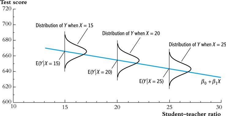
Figure 1. simple linear regression model

① β₀ : y intercept 

② β₁ : slope or coefficient on X 

○ also called parameter, regression coefficient, weight, etc 

○ intuitively, elasticity means the degree to which the absolute value of the slope is large

○ in microeconomics, elasticity means the slope multiplied by (-1).

③ types of regression lines

○ population regression line: regression line obtained from the characteristics of the population

○ fitted regression line: regression line obtained from the characteristics of the sample

④ u_i : residual

⑤ difference between residual and error

○ the errors mentioned in the future actually mean residuals

⑥ characteristic of variance 

○ homoscedasticity: VAR(u_i | X_i) and Xi are independent. an impractical assumption. default setting for many statistical programs

○ heteroscedasticity **: VAR(u_i | X_i) depends on X_i

○ (note) a model with homoscedasticity is a good model 

⑶ assumptions 

① assumption 1. X_i does not provide any information about the error

○ if there is a pattern on a residual plot, the model is not a good model 

② assumption 2. (X_i, y_i) is i.i.d. 

③ assumption 3. the existence of 4^th order moment

⑷ induction of the fitted regression line  

① method 1. method of moment estimator (MOM) or sample analog estimation 

○ calculation process

② method 2. method of least squares or ordinary least squares (OLS)

○ definition: calculate the minimum value of sum of squares of the errors (SSE)

○ provided by all statistical softwares 

○ calculation process : if X_i is one-dimensional 

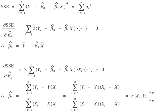
○ method of least squares is based on maximum likelihood estimation (assuming the residual has homoscedasticity and normality)

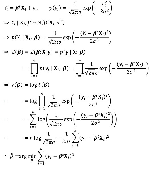
○ the regression of X to Y and the regression of Y to X are generally not the same

○ E(X₂), E(XY), E(X), ect are involved in the regression of X to Y

○ E(Y₂), E(XY), E(Y), etc are involved in the regression of Y to X

○ E(X₂), E(Y₂), ect make the asymmetry

③ Method 3. Cross entropy 

○ general definition 

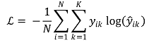
○ binary classification

○ if y is represented as one-hot vector [0, ···, 1, ···, 0], the following is established 

⑸ Characteristics of regression line 

① Overview

② Unbiasedness

③ Efficiency

○ Gauss-Markov theorem: OLS is efficient when homoscedasticity is satisfied  

④ Consistency

⑤ Asymptotic normality

○ slope

○ y intercept - heteroscedasticity-robust standard error

○ y intercept - homoscedasticity-robust standard error

⑹ evaluation of the regression line

① criterion 1. linearity 

② criterion 2. homoscedasticity : residual terms having equal variances

③ criterion 3. normality : residual terms following normal distribution

○ Box-Cox : In cases where it is difficult to assume normality in linear regression models, this method transforms the dependent variable to be closer to a normal distribution.

⑺ coefficient of determination : also called R-squared

① coefficient of determination R2

○ definition

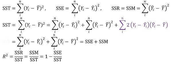
○ SST : total variation

○ SSR : variation for regression equation

○ SSE : variation due to error

○ SSE is also called residual sum of squares (RSS), sum of squared residuals (SSR)

○ reason why the term ■ is 0: because covariance of bias and chance error is intuitively 0

○ meaning

○ meaning 1. the proportion of the variance of Y that X can describe (no units)

○ meaning 2. the sum of squares described by the regression line ÷ the total sum of squares

② the coefficient of determination is the same as the square of the correlation coefficient

③ Fraction of the variance unexplained (FVU)

④ characteristics 

○ 0 ≤ R² ≤ 1

○ the closer R² is to 1, the better the goodness of fit of regression line is

○ estimator of β₁ = 0 ⇒ R² = 0

○ R² = 0 ⇒ estimator of β₁ = 0 or X_i = constant

⑻ average error regression

① formula for SSE 

② the expected value of SSE

○ total degree of freedom = degree of freedom of residual + degree of freedom of regression line

○ total degree of freenom = n-1

○ degree of freedom of regression line = 1 (∵ there is only one regression variable)

○ degree of freedom of residual = n-2 

③ Mean squared error (MSE)

④ Standard error regression (SER)

⑤ SSE and unbiased estimator of variance

⑼ Example 1. the etymology of regression

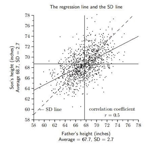
Figure 2. the etymology of regression

① X : a father’s height

② Y : a son’s height

③ E(X) = 67.7, E(Y) = 68.7, σ_X = 2.7, σ_Y = 2.7, ρ_XY = 0.5 

④ E(Y | X = 80) = 74.85

⑤ E(Y | X = 60) = 64.85

⑥ conclusion

○ the son of a tall father tends to get shorter

○ the son of a short father tends to grow taller

○ finally, the son’s height tends to return to the average

○ however, since the above tendency is only based on expected value, the variance of sons’ generation’s height is not necessarily lower than the variance of fathers’ generation’s height 

⑽ example 2. predicting Y-values outside the range of independent variables: also called extrapolation

① generally, it is unadvisable to use extrapolation 

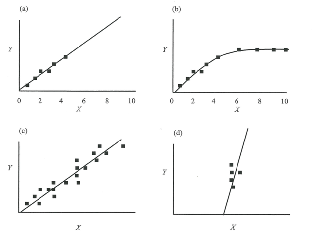
Figure 3. problems of extrapolation

② extrapolation methodology is not always wrong

○ example: research on biological evolution

⑾ Example problems for linear regression and bivariate normal distribution

⑿ Python code

from sklearn import linear_model 
reg = linear_model.LinearRegression() 
reg.fit([[0, 0], [1, 1], [2, 2]], [0, 1, 2])
# LinearRegression() 
reg.coef_ 
# array([0.5, 0.5])

3. multiple linear regression model  

⑴ definition: the case of a multiple regression analysis in which the dependency is shown as a linear function  

⑵ omitted variable bias 

① definition : a phenomenon in which the expected value of the error is not zero due to omitted variables

○ endogenous variable: variables correlated with ui  

○ exogenous variable: variables uncorrelated with ui  

② condition 1. omitted variables and regressor (e.g., X_i) should have correlation

③ condition 2. omitted variables should be determinators of Y

④ the convergent value of the slope

○ ρ_Xu ＞ 0 : upward bias

○ ρ_Xu ＜ 0 : downward bias

⑤ if the value of the coefficient changes significantly when a new variable is added, it can be said that there is omitted variable basis

⑶ representation of data

① unbiasedness, consistency, and asymptotically jointly normal are observed in the above estimators 

② robustness : a characteristic that adding a new regressor does not significantly change any slope value of a regressor 

③ sensitivity : a characteristic that adding a new regressor significantly changes the slope value of a particular regressor 

⑷ assumptions

① assumption 1. error is not explained by X_1i,, ···, X_ki

② assumption 2.** (X_1i, ···, X_ki,Y_i) is i.i.d.  

③ assumption 3. existence of 4th order moment

④ assumption 4. no perfect multicollinearity 

○ multicollinearity : a characteristic that the linear combination of one independent variable and another independent variable is highly correlated

○ (note) multiple linear regression model expects independent variables to be truly independent 

○ perfect multicollinearity: if one regressor has perfect linearity with the other regressors. the determinant value = 0

○ perfect multicollinearity is not the nature of a variable, but the nature of a data set

○ when you attempt a regression analysis on perfect multicollinear data, the number of possible coefficients is infinite: impossible to perform regression analysis 

○ imperfect multicollinearity : two or more regressors are just highly correlated

○ not a problem at once

○ the variance of the slope estimator is quite large → difficult to trust the slope estimator

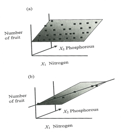
Figure 4. the reason why multi-collinearity increases the variance of the slope estimator

⒝ a variety of planes may exist within the significance interval

○ in general, a pair of variables should not have a correlation of more than 0.9

○ solution

○ draw pairwise plots of all combinations and remove highly correlated variables

○ PCA, weighted sum, etc. may be attempted, but each has its own shortcomings

○ (note) R Studio randomly ignores the last of the problematic terms when analyzing perfect multicollinearity data

⑸ OLS estimator: determine the coefficient by calculating the following simultaneous equations 

⑹ characteristics of the regression line

① unbiasedness

② consistency 

③ asymptotically jointly normality

④ Frisch-Waugh theorem 

⑺ adjusted R²

① drawbacks of R² : the degree of fitting is not well reflected in multiple regression model

○ drawback 1. R² always increases whenever a new regressor is added because the minimum value of SSE is reduced

○ drawback 2. high R² does not verify the absence of omitted variable bias  

○ drawback 3. high R² does not verify the current regressors are optimal 

○ to resolve drawback 1, adjusted R2 is introducted

② formula

③ characteristic 

○ adjusted R² ≤ R²

○ adjusted R² can be negative

○ The value decreases as inappropriate variables are added

⑻ standard error regression (SER): k is the number of independent variables in the regression equation

⑼ joint hypothesis: hypothesis when there are more than or equal to 2 constraints

① idea 1. t1 and t2 are independent

② idea 2. t₁ and t₂ have multicollinearity

③ general case

○ in general, heteroscedastic-robust F-statistics is used

○ many statistical programs take homoscedastic-robust F-statistics as default setting

④ null hypothesis 

⑽ redefinition of multiple linear regression model 

① H₀ : if you want to test β₁ = β₂,  

② H₀ : if you want to test β₁ + β₂ = 1, 

⑾ conditional mean independence

① definition

② X_1i is not correlated with ui for given X_2i 

③ β₂ may not have consistency: but it is not important 

⑿ matrix notation

① linear regression model

○ for a scalar Y, column vector X, and β, 

○ generalization

② assumption

○ assumption 1. E(ui

Xi) = 0

○ assumption 2. (X_i, Y_i), i = 1, ···, n is i.i.d. 

○ assumption 3. X_i and u_i have nonzero finite fourth moment 

○ assumption 4. 0 ＜ E(X_iX_i^t) ＜ ∞, no perfect multicollinearity 

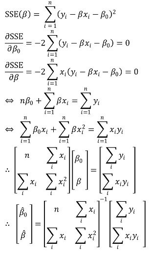
③ OLS modeling - a simple version

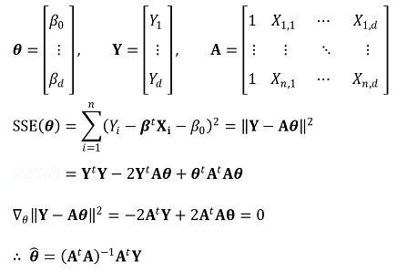
④ OLS modeling

⑤ consistency

⑥ multivariate central limit theorem

⑦ asymptotic normality

⑧ robust standard error (Eicker-Huber-White standard error)

⑨ robust F

Input: 2019.06.20 23:26